10 Analytically reproducible documents

When in RStudio, quickly jump to this page using r3::open_reproducible_documents().

Session objectives:

Learn what a reproducible document is, how R Markdown achieves being reproducible, and why it can save you time and effort
Write and use R code within a document, so that it will automatically insert the R output into the final document.
Learn about and use Markdown formatting and syntax for writing documents.
Learn about and create different document types like HTML or Word from an R Markdown document.

10.1 Why try to be reproducible?

Take about 5 min to read over this section.

Both reproducibility and replicability are cornerstones for doing rigorous and sound science. As we’ve learned, reproducibility in science is fairly lacking, which this course aims to fill. But being reproducible isn’t just about doing better science, it can also:

Make you much more efficient and productive, as less time is spent between coding and putting your results in a document (e.g. no need to copy and paste).
Make you more confident in your results, since what you report and show as figures or tables will be exactly what you get from your analysis. Again, no copying and pasting required!

Hopefully by the end of this session you’ll try to start using R Markdown files for writing your manuscripts and other technical documents. Believe us, after you’ve learned how to incorporate text with R code, it can save so much time in the end, and make your analysis and work more reproducible. Plus you can create some very aesthetically appealing reports, way more easily than you could if you did it in Word.

10.2 Creating an R Markdown file

Take about 5 min to read over the next few paragraphs.

R Markdown is a file format (a plain text format like R scripts or .csv files) that allows you to be more reproducible in your analysis and to be more productive in general in your work. R Markdown is a extension of Markdown that integrates R code with written text (as Markdown formatting).

So what is Markdown? It is a markup syntax and formatting tool, like HTML, that allows you write a document in plain text that can then be converted into a vast range of other document types, e.g. HTML, PDF, Word documents, slides, posters, or websites. In fact, this website is built from R and Markdown! (Plus other things like HTML.) The Markdown used in R Markdown is based on pandoc (“pan” means all and “doc” means document, so “all documents”). Pandoc is a very powerful, popular, and well-maintained software tool for document conversion. But, we’ll get to Markdown more a bit later. For now we’re going to focus on the main reason to use it: for incorporating R code and output into a document! By using R code in a document, you can have a seamless integration between document writing and doing your analysis.

Why would you use this? There are many reasons, some of them being:

There is less time between exploring a new dataset or analysis and sharing your findings with collaborators, because the writing and documenting is woven in with your R analysis code.
If you finish an analysis and produce a report, but later find out there are problems with the data or you get new data, updating your report is as easy as clicking a button to regenerate it.
How you got and present your results is based on the exact sequence of steps given in your R Markdown document, so showing others on how the analysis is done is easy because the how is explicitly shown in the document.
Likewise, by reading others’ R Markdown documents, it is easier to learn what was done in their analysis because the logic and sequence is shown in the document itself.

Let’s go over this together.

Ok, let’s create and save an R Markdown file. Go to “File -> New File -> R Markdown”, and a dialog box will then pop up. Type in “Reproducible documents” in the title section and your name in the author section. Choose HTML as the output format. Then save this file as rmarkdown-session.Rmd in the doc/ folder.

We now have an R Markdown file. Inside the file, there is some text that gives a brief overview of how to use it. For now, let’s ignore the text.

At the top of the R Markdown file, you will see something that looks a bit like this:

---
title: "Reproducible documents"
author: "Your Name"
date: "6/18/2020"
output: html_document
---

This section is called the YAML header and it contains commands and metadata about the document. Most Markdown documents have this YAML header at the top of the document and they are always surrounded by --- on the top and bottom of the section. YAML is a data format that has the form of a key: value pairing to store data. The keys in this case are title, author, date, and output. The values are those that follow the key (e.g. “Your Name” for author). In the case of R Markdown, these key data are used to store the settings that R Markdown will use to create the output document. The keys listed above are some of many settings that R Markdown has available to use.

In the case of this YAML header, the R Markdown document will generate an HTML file because of the output: html_document setting. You can also create a word document with output: word_document. While PDF documents are also able to be created, they require installing LaTeX through the R package tinytex, which can sometimes be complicated to install. So we will only cover HTML and Word documents in this session.

So how do we create an HTML (or Word) document from the R Markdown document? By “knitting” it! At the top of the pane near the save button, there is a button with the word “Knit” and yarn beside it, as shown in Figure 10.1. To knit, you either click that button or by typing “Ctrl+Shift+K” anywhere in the R Markdown document.

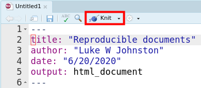
Figure 10.1: Location of the Knit button in RStudio.

When you click it, a bunch of commands should pop up in a new pane called “R Markdown”, followed by a new window popping up with the newly created document. Alternatively, the HTML document may pop up in the “Viewer” pane.

Cool, so now you’ve created an HTML document! Let’s try making a Word document. Change the YAML value in the key output: from html_document to word_document. Then knit the document again (with the “Knit” button or with “Ctrl-Shift-K”). Now, a Word document should open up. This is the basic approach to creating documents from R Markdown.

10.3 Exercise: Create another R Markdown document.

Time: 5 min

Create another R Markdown document using RStudio’s interface.
- Write the title as “Trying out R Markdown”.
- Choose “HTML” as the document type.
Save the document in the doc/ folder and name it another-one.Rmd.
Knit the document with either “Ctrl-Shift-K” or with the RStudio “Knit” button.
Look at the output document, then change the YAML value for the output: key from html_document to word_document. Knit again.
Open the Word file if it hasn’t been opened already.

10.4 Inserting R code into your document

Being able to insert R code directly into a document is one of the most powerful characteristics of using R Markdown. This frees you from having to switch between programs when writing text and when running R code in order to obtain an output that you’d then put into the document.

Running and including R code in R Markdown is done through “R code chunks”. You insert these chunks into the document by either typing “Ctrl+Alt+I” or using the menu item “Code -> Insert Chunk”, with the cursor at the location you want the chunk to be. Before we do that, delete all the text in your R Markdown document (the rmarkdown-session.Rmd file), excluding the YAML header. Make sure that the YAML key output: is set to html_document.

Then, place your cursor two lines below the YAML header and insert a code chunk (“Ctrl+Alt+I” or “Code -> Insert Chunk”). The code chunk should look something like this:

```{r}
 
```

In the code chunk, type out 2 + 2, so it looks like:

```{r}
2 + 2 
```

You can run R code inside the code chunk the same as you would when in an R script. Typing “Ctrl+Enter” on the line will send the code 2 + 2 to the console, putting the output directly below the code chunk in the R Markdown document. This output though is temporary.

To get it inserted into the HTML document, knit (“Ctrl+Shift+K”) the document and see what happens in the created HTML document. The output 4 should appear below the code chunk in the HTML document. Something like this:

2 + 2
#> [1] 4

This is a very simple example of how code chunks work. Normally, things are more complicated than this though. Usually we have to load R packages to use for running R, and this is no different in an R Markdown document. Create a new code chunk and then type setup right after the r. It should look like:

```{r setup}

```

This area that you typed in is for code chunk labels. In this case, we labelled the code chunk with the name setup. Code chunk labels should be named without _, spaces, or . and instead should be one word or be separated by -. An error may not necessarily occur if you don’t follow this rule, but there can be unintended side effects that you may not realize and R will likely not tell you about it, probably causing you quite a bit of annoyance and frustration.

A nifty thing about using chunk labels is that you can see the name when using “Document Outline” (found using “Ctrl+Shift+O”), but only if you have the option set in the “Tools -> Global Options -> R Markdown -> Show in document outline”.

The name setup is also a special name for R Markdown. When you run other code chunks in the document, if the document was just opened up, R Markdown will first run the code in the setup chunk. This is a good place to put your library() calls. Let’s add tidyverse and NHANES to the chunk:

```{r setup}
library(tidyverse)
library(NHANES)
```

Let’s add another code chunk, and this time simply put NHANES in it:

```{r}
NHANES
```

You can run this code normally, with the cursor over the code and typing “Ctrl+Enter”. Or we can knit (“Ctrl+Shift+K”) the document and see what it looks like. When the HTML document opens, you should see some text below the setup chunk that might look something like this:

Registered S3 methods overwritten by 'dbplyr':
  method         from
  print.tbl_lazy     
  print.tbl_sql      
── Attaching packages ─────────────────────────────────────────── tidyverse 1.3.0 ──
✓ ggplot2 3.3.2          ✓ purrr   0.3.4     
✓ tibble  3.0.1          ✓ dplyr   1.0.0.9000
✓ tidyr   1.1.0          ✓ stringr 1.4.0     
✓ readr   1.3.1          ✓ forcats 0.5.0

You probably don’t want this text in your generated document. You can change how code chunks work by using chunk options. They are available either by clicking on the gear in the top right corner of the chunk (shown in Figure 10.2) or by typing in the area after the chunk label section.

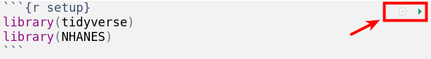
Figure 10.2: Changing the settings for the code chunk actions.

So, if you want to run the code but not show those messages and warnings, you can add the options message=FALSE and warning=FALSE:

```{r setup, message=FALSE, warning=FALSE}
library(tidyverse)
library(NHANES)
```

If you want to hide the code, the messages, the warnings, and the output, but still run the code, you use the option include=FALSE.

```{r setup, include=FALSE}
library(tidyverse)
library(NHANES)
```

Other common options are:

echo: To show the code. The default value to show is TRUE, to hide is FALSE.
results: To show the output results. The default is 'markup', to hide is 'hide'.
eval: To evaluate (to run) the R code in the chunk. The default value is TRUE and FALSE does not run the code.

These options all work on the individual code chunk. Note, that all the chunk options must be on one line, after the {r tag. If you want to set an option to all the code chunks, for instance to hide all the code but keep the output, you use the function knitr::opts_chunk$set(echo = FALSE). We won’t do this in this session, but here is what it looks like:

```{r setup}
library(tidyverse)
library(NHANES)
knitr::opts_chunk$set(echo = FALSE)
```

A common results output that is included in documents are tables. So let’s run some R code and get R Markdown to create one. First, create a new code chunk and name it mean-bmi-table. Then, let’s copy the code from the Data Wrangling session, from Section 7.15, and include the pivot_wider() continuation of the pipe. To keep the output smaller, we’ll only select SurveyYr, Sex, BMI, and Age.

```{r mean-bmi-table}
NHANES %>%
    rename(Sex = Gender) %>%
    select(SurveyYr, Sex, BMI, Age) %>%
    pivot_longer(c(-SurveyYr, -Sex),
                 names_to = "Variables",
                 values_to = "Values") %>%
    group_by(SurveyYr, Sex, Variables) %>%
    summarize(MeanValues = mean(Values, na.rm = TRUE)) %>%
    pivot_wider(names_from = Variables, values_from = MeanValues)
```

#> # A tibble: 4 x 4
#> # Groups:   SurveyYr, Sex [4]
#>   SurveyYr Sex      Age   BMI
#>   <fct>    <fct>  <dbl> <dbl>
#> 1 2009_10  female  38.0  27.0
#> 2 2009_10  male    35.5  26.7
#> 3 2011_12  female  37.3  26.5
#> 4 2011_12  male    36.2  26.4

This output is almost in a table format. We have the columns that could be the table headers, and we have rows that would be meaningful table rows too. To convert it into a pretty table in the R Markdown HTML output document, we use the kable() function from the knitr package. Because we don’t want to load all of the knitr functions, we’ll use knitr::kable() instead.

```{r mean-bmi-table}
NHANES %>%
    rename(Sex = Gender) %>%
    select(SurveyYr, Sex, BMI, Age) %>%
    pivot_longer(c(-SurveyYr, -Sex),
                 names_to = "Variables",
                 values_to = "Values") %>%
    group_by(SurveyYr, Sex, Variables) %>%
    summarize(MeanValues = mean(Values, na.rm = TRUE)) %>%
    pivot_wider(names_from = Variables, values_from = MeanValues) %>% 
    knitr::kable(caption = "Table caption. Mean values of Age and BMI for each sex by survey year.")
```

Table 10.1: Table caption. Mean values of Age and BMI for each sex by survey year.
SurveyYr	Sex	Age	BMI
2009_10	female	38.01545	27.04892
2009_10	male	35.51192	26.70107
2011_12	female	37.26733	26.49190
2011_12	male	36.15090	26.39708

Now, knit (“Ctrl+Shift+K”) and view the output in the HTML document. Pretty eh!

10.5 Exercise: Creating a table using R code

Time: 10 min

In the doc/another-one.Rmd, create a new code chunk and call it setup. Include the library() functions to load tidyverse and NHANES.
Create another code chunk and call it prettier-table. Copy the code from above that calculates the mean BMI and Age and paste the code into the new chunk.
Using the function round() around the mean() function, round the values to 1 digit.
Rename SurveyYr to Year by using rename() after the pivot_wider().
After the rename() function, use mutate() to modify the Sex column so that male and female get capitalized. Use str_to_sentence(Sex) to capitalize the first letter of the word.
Inside the previous mutate() function, modify the Year column to replace the _ with - by using str_replace(Year, "_", "-").
Run the code chunk to make sure the code works, then knit the document. Don’t forget about including the knitr::kable() function at the end of the pipe.

10.6 Formatting text with Markdown syntax

Formatting text in Markdown is done using characters that are considered “special” and act like commands. So these special characters indicate what text is bolded, what is a header, what is a list, and so on. Almost every feature you need to write a scientific document is available in Markdown, though not all. If you can’t get Markdown to do what you want, my suggestion would be to try to fit your writing around Markdown, rather than force or fight with Markdown to do something it wasn’t designed to do. You might actually find that the simpler Markdown approach is easier than what you wanted or were thinking of doing, and that you can actually do quite a lot Markdown’s capabilities.

10.6.1 Headers

Creating headers (like chapters or sections) is done by using one or more # at the beginning of a line and should always be preceded and followed by an empty line:

# Header 1

Paragraph.

## Header 2

Paragraph.

### Header 3

Paragraph.

10.6.2 General text formatting

**bold** gives bold.
*italics* gives italics.
super^script^ gives super^script.
sub~script~ gives sub_script.

10.6.3 Lists

Lists are created by adding either - or 1. to the beginning of a line and an empty line must be at the start and end of the list.

For unnumbered lists, it looks like:

- item 1
- item 2
- item 3

which gives…

item 1
item 2
item 3

And numbered lists look like:

1. item 1
2. item 2
3. item 3

which gives…

item 1
item 2
item 3

10.6.4 Block quotes

Block quotes are used when you want to emphasize a block of text, usually for quoting someone. You create a block quote by putting a > at the beginning of the line, and as with the lists and headers, needs empty lines before and after the text. So it looks like:

> Block quote

which gives…

Block quote

10.6.5 Adding footnotes

Footnotes are added by enclosing a number or word in square brackets ([]) and beginning with an uptick (^). It looks like:

Footnote[^1] or this[^note].

[^1]: Footnote content
[^note]: Another footnote

which gives…

Footnote¹ or this².

10.6.6 Adding links to websites

Including a link to a website in your document is done by surrounding the link text with square brackets ([]) followed by the link URL in brackets (()). There must not be any space between the square brackets and the regular brackets (it should look like []()).

[Link](https://google.com)

which gives…

Link

10.6.7 Inserting (simple) tables

While you can insert tables using Markdown too, it isn’t recommended to do that for complicated or large tables. Tables are created by separating columns with |, with the table header being separated by a line that looks like |:--|. A simple example is:

|   | Fun | Serious |
|:--|----:|--------:|
| **Happy** | 1234 | 5678 |
| **Sad** | 123 | 456 |

which gives…

	Fun	Serious
Happy	1234	5678
Sad	123	456

The |---:| or |:---| tell the table to left-align or right-align the values in the column. Center-align is |:----:|.

So you can probably imagine, doing this for larger or even slightly more complicated tables is not practical. A good alternative approach is to create the table in a spreadsheet, importing that table into R within a code chunk, and using knitr::kable() to create the table after that.

10.6.8 Inline R code

R Markdown also allows you to including numbers (or other output) directly into a paragraph. For instance, if you want to add a mean into some text, it would look like:

The mean of BMI is `r round(mean(NHANES$BMI, na.rm = TRUE), 2)`.

which gives…

The mean of BMI is 26.66.

But note that using inline R code can only insert a single number or character value, nothing more.

10.7 Exercise: Practice using Markdown for writing text

Time: 8 min

Create three level 1 headers (#), called “Intro”, “Methods and Results”, “Discussion”.
Create a level 2 header (##) under “Methods and Results” called “Analysis”.
Write one random short sentence under each header. Bold (**word**) one word in each and italicize (*word*) another.
Include an inline R code to calculate 10 divided by 2 in the “Analysis” section.
Play around with adding some lists, tables, or anything else.

10.8 Inserting figures, as files or from R code

Aside from tables, figures are the other most common form of output inserted into documents. And like tables, you can insert figures into the document either with Markdown or with R code chunks. Let’s first try doing it with Markdown. First, we need an image to use. Open a browser and search for a picture to use (we’re using a kitten, because they’re cute). Download the image, create a folder in doc/ called images, and save the image in that folder. Then in your R Markdown document, use the Markdown syntax for images: ![Caption text](path/to/image.png). The image can be png, jpeg, or pdf. If you download an image and intend to use it in an official document, you will need to add text on the source and author of the image.

![Image by Dimitri Houtteman from Pixabay.](doc/images/kitten.jpg)

Which gives…

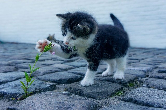
Image by Dimitri Houtteman from Pixabay

You can also directly include a link to a picture instead of downloading the image, though this may only work in HTML documents and only if you have internet access.

Markdown syntax to control the image is limited. If you want to change the size of the image, it can be difficult. However, using R code chunks can simplify this!

First, let’s create a new code chunk (“Ctrl+Alt+I”), name the code chunk kitten-image, and add the function knitr::include_graphics(). To make it easier to find the image, use here::here() to point to the picture. It should look like this:

```{r kitten-image}
knitr::include_graphics(here::here("doc/images/kitten.jpg"))
```

Knit the document again (“Ctrl+Shift+K”) and view the HTML document with the new picture. Now, let’s change the width and height of the image, along with adding a figure caption. We do this with these code chunk options:

fig.cap: For writing the figure caption.
out.width and out.height: Sets the image width and height for external images (not created by R). Can use percent to set the size, e.g. "75%".

Change the width and height to "50%", along with adding a caption like "Kittens attacking flowers!":

```{r kitten-image, out.width="50%", out.height="50%", fig.cap="Kittens attacking flowers!"}
knitr::include_graphics(here::here("images/kitten.jpg"))
```

Figure 10.3: Kittens attacking flowers!

Knit again to see how the image changed. Great! But the real fun comes by inserting figures directly from R code. Let’s create another code chunk (“Ctrl+Alt+I”) and name the code chunk exploring-plot. We’ll copy and paste the visualization code we used in Section 9 into the code chunk. You can copy and paste this code as well:

```{r exploring-plot}
nhanes_tidied <- NHANES %>% 
    rename(Sex = Gender) %>% 
    filter(!is.na(Diabetes))
nhanes_tidied %>% 
    ggplot(aes(x = BMI, y = BPSysAve, colour = Age)) +
    geom_point() +
    facet_grid(cols = vars(Diabetes),
               rows = vars(Sex)) +
    scale_color_viridis_c() +
    theme_minimal()
```

nhanes_tidied <- NHANES %>% 
    rename(Sex = Gender) %>% 
    filter(!is.na(Diabetes))
nhanes_tidied %>% 
    ggplot(aes(x = BMI, y = BPSysAve, colour = Age)) +
    geom_point() +
    facet_grid(cols = vars(Diabetes),
               rows = vars(Sex)) +
    scale_color_viridis_c() +
    theme_minimal()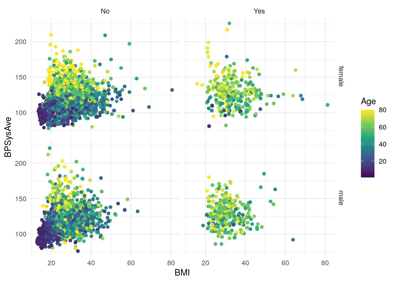

Run the code in the code chunk to make sure it runs properly, by typing “Ctrl+Enter” (or “Ctrl+Shift+Enter” to run all the code in the code chunk at once). Once it creates the figure below the code chunk, knit the document again to see how the figure gets inserted into the HTML document.

You might also notice that you get a warning below the code chunk too. Let’s get rid of that warning message, make the figure bigger, and add a caption. When you create a figure with R code, you need to use different options instead of out.width and out.height:

fig.width and fig.height: Sets the width and height of the figure, where the default value is 7.

Add the chunk options fig.width, fig.height, and fig.cap, along with the warning=FALSE to the code chunk.

```{r exploring-plot, fig.width=9, fig.height=8, fig.cap="Exploratory figure of the NHANES dataset", warning=FALSE}
nhanes_tidied <- NHANES %>% 
    rename(Sex = Gender) %>% 
    filter(!is.na(Diabetes))
nhanes_tidied %>% 
    ggplot(aes(x = BMI, y = BPSysAve, colour = Age)) +
    geom_point() +
    facet_grid(cols = vars(Diabetes),
               rows = vars(Sex)) +
    scale_color_viridis_c() +
    theme_minimal()
```

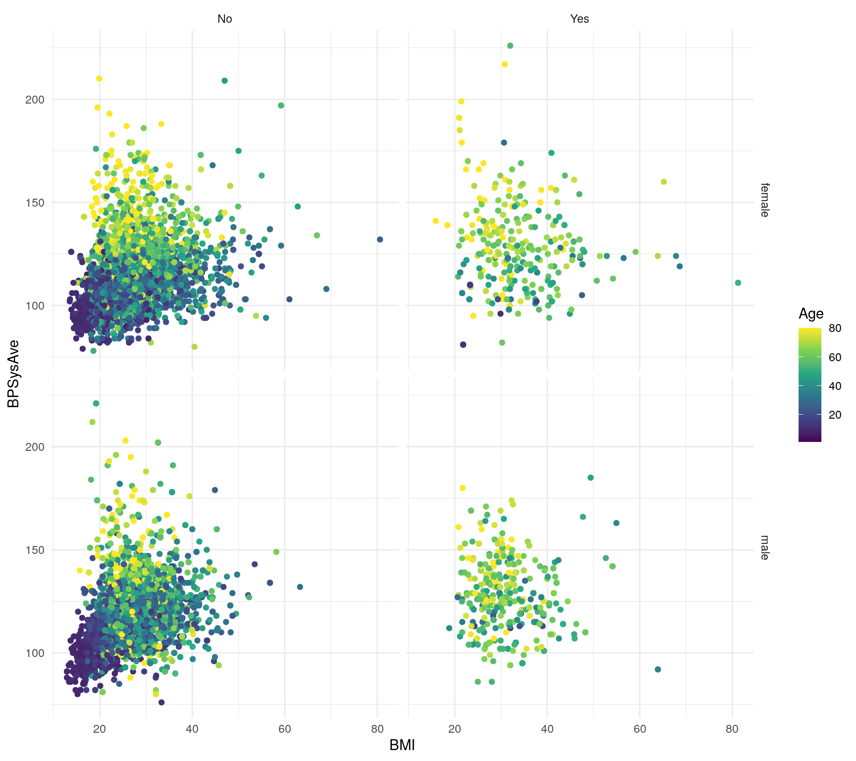
Figure 10.4: Exploratory figure of the NHANES dataset

Knit the document again and view the generated HTML document. Cool! You’ve just made an easily reproducible figure in a document!

10.9 Other R Markdown features

Take 5 min to read these sections below before proceeding to the final exercise.

10.9.1 Making your report prettier

For HTML documents, customizing the appearance (e.g. fonts) is pretty easy, since settings to change the theme can be used directly in the YAML header. For instance, there’s a setting within html_document called theme. It would look like this:

---
title: "My report"
output:
    html_document:
        theme: sandstone
---

Notice the indentations. Indentation tells YAML what key is related to another key, i.e. if it is a sub-key. The key theme is a sub-key (an option) of html_document, which is a sub-key (an option) of output. Check out the R Markdown documentation to see other themes you can use. The themes are all Bootswatch themes, with most of them being available for use in HTML documents.

Modifying the theme and appearance of Word documents, on the other hand, is much more difficult. Since Word can’t easily be programmatically modified like HTML can, changing the appearance of the document itself requires that you manually create a Word template file first, manually modify the appearance, and then link to that template file with the reference_docx option in the YAML header (as a sub-key of word_document). More detail on this can be found in the documentation.

10.9.2 Collaborating on R Markdown documents

There are multiple ways in general of collaborating on a document:

One person has the primary task of writing up the report and then gets feedback from other collaborators through the use of “Track Changes” or by inserting comments in Word.
Multiple people are responsible for writing the report and probably use different documents that they will end up merging later on. Or they email back and forth (or use something like Dropbox or shared folders) and work on a single document.

The first workflow is not possible in an R Markdown document. Instead, you’d use a workflow that probably resembles how peer reviews are done, i.e. reading the document and making comments in a separate file to upload to the journal later. Or you’d use a workflow that revolves around GitHub and Git, an efficient workflow that has been tried and tested by tens of thousands of teams in tens of hundreds of companies globally. The goal of this course is to slowly move researchers more into the modern era, based on modern technology, tools, and workflows.

The second workflow is pretty similar. You might split up a document into sections that each collaborator may work on, and then later on merge them together. This last approach is what we will get you to do for the group project.

10.10 Final exercise: Group work

Time: 30 min

It’s now time to start putting things together as a report and to present on it later in the afternoon.

As a team, complete item 7 and its sub-tasks in the group assignment (to jump quickly to the assignment, run r3::open_assignment() in the RStudio Console).
Distribute the tasks so each team member is (mostly) doing something different.
- Create one R Markdown file for each team member, and each person works on their own file. Later this file will be merged into the final report.
Frequently use the “Git workflow”: Add to staging, commit, push, and pull the changes you’ve made.
- You’ll likely deal with merge conflicts, which is a good chance to practice with Git more.
Try to “knit” your document to HTML often, to make sure the analysis is reproducible.
- Note: For now, do not add and commit the HTML report.

Once you as a team are happy with the report, figures, and tables, make sure that everyone does a final add-commit-push to your GitHub repository. Then, designate someone to pull from GitHub, merge each R Markdown file into a single report.Rmd file in the doc/ folder, and knit the .Rmd document to make sure it knits correctly. Then add-commit-push the HTML report to GitHub. You should now be ready to present your report!

Footnote content↩︎
Another footnote↩︎